Daniel N. Bassett, Qi Shao, Daniel L Benoit, Kurt T. Manal, Thomas S. Buchanan
Center for Biomedical Engineering Research
University of Delaware
Newark, DE
INTRODUCTION
The implementation of biomechanical EMG-driven models has become more widespread in recent years. One important application for such modeling is in the analysis of muscle forces during gait. Such models generally focus on a single joint (i.e., the knee or ankle) due to the problems of collecting EMGs from so many muscles. However, although the models must balance the forces for any particular joint, models that take into account multiple joints simultaneously may yield different solutions due to the way biarticular muscles are reckoned.
In this study, we present an expanded version of our model that allows us to account for multiple joints. We used this model to predict joint moments for the ankle and the knee in two ways: treating each of the joints separately and treating them both together. We then compared the results obtained using these two methods to evaluate the differences in the prediction of joint moments and muscles forces.
METHODS
Data Collection
For this preliminary study, we collected data from one healthy individual possessing a normal gait pattern and moderate physically active background. The subject performed multiple maximum voluntary contractions (MVC) and gait trials. Kinematic data were recorded using a Qualysis motion system. Ground reaction forces were obtained by means of an in-floor force plate, and activity from nine muscles was recorded using electromyography (EMG). The muscles about the knee were chosen in accordance with Lloyd [1] and included the semitendinosus, biceps femoris, rectus femoris, vastus lateralis, vastus medialis, gastrocnemius lateralis, and gastrocnemius medialis. For muscles about the ankle, EMGs were collected from the soleus (Sol) and tibialis anterior (TA) beyond the medial and lateral gastrocnemii (GM and GL) already included at the knee.
Data Processing
In addition to the nine muscles we collected from, we averaged the EMG for the medial and lateral vasti to obtain data for the vastus intermedius. Also, the biceps femoris was assumed to have the same EMG for the long head and short head.
The EMG was relieved of bias, then rectified, high-pass filtered, low-pass filtered, and normalized by the maximal activation from the MVC trials, giving us vales we termed “EMG activation” [2].
The kinematic data were used to calculate joint angles for the hip, knee, and ankle, from which muscle tendon lengths and muscle moment arms were determined using SIMM for each of the eleven muscles analyzed. Furthermore, the kinematic data in combination with the ground reaction forces were used to estimate joint moments by inverse dynamics.
Biomechanical Model
The model we use is forward dynamic and EMG-driven based on a Hill-type model which includes active, passive, and damping components [3].
 (1)
(1)Equation (1) displays the relationship between the three components, and includes muscle force (F), max isometric force (Fmax), active force (FA), velocity dependent force (FV), passive force (FP), muscle activation (a(t)), muscle fiber length (lm), muscle fiber velocity (vm), damping (bm), and pennation angle (φ).
Muscle activation was obtained by passing EMG activation through a history dependent recursive filter and then non-linearizing it. Muscle fiber length was then calculated by using a forward integration based on equation (1), and recalling that the force passing through the tendon must be equal to that produced by the muscle. Once the muscle fiber length is known it was subtracted from the muscle tendon length giving the length of the tendon. Tendon force was interpolated using the corresponding force-length relationship. Finally, joint moments can be easily obtained from muscle forces and muscle moment arms.
Subject specific muscle parameters such as tendon slack length are difficult to measure accurately in vivo. For this reason we converted our forward dynamic model into a hybrid model during the tuning process and tuned these parameters for each subject (within physiological bounds). Model parameters were adjusted using an optimization algorithm [4] so that the joint moments calculated from inverse dynamics matched those of the forward dynamic calculations. Model tuning was performed three different times on the first trial: ankle, knee, and ankle and knee combined. The calibrated models were then used for joint moment predictions on novel data.
results &Discussion
Analysis of the joint moments produced by applying the three different calibrations revealed consistency in the model’s predictions. Tuning the model with two joints simultaneously as opposed to one increased the error a modest amount. In Figure 1, it can be seen that the joint moment patterns are closely correlated. The R2 values were 0.97 for the individual optimization and 0.96 for the combined calibration; the RMS errors were 7.7% and 8.1% respectively. The difference between the two predictions was 1.3% (RMS) for the ankle.
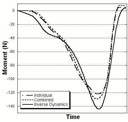
Figure 1. Ankle Joint Moment Comparison
The differences in estimated forces for muscles around the ankle are shown in Figure 2. The different optimizations resulted in little deviation in muscle force estimation between the soleus and tibialis anterior. However, the gastrocnemii force predictions were on average between 15 and 20 percent different between calibrations. The RMS deviations showed a decrease in force from individual to combined tuning of 170 N for the GM and 13 N for the GL.
This study showed that our model was able to estimate joint moments when accounting for multiple joints with similar accuracy as
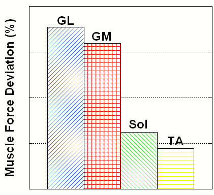
Figure 2. Muscle Force Deviation between Ankle and Combined Ankle and Knee Optimizations
when only examining a single joint. More importantly, however, is the model’s ability to predict muscle forces. The force deviations between ankle joint and combined calibration were more evident in the GM and GL compared to the Sol and TA. This was expected since the gastrocnemii are the only biarticular muscles spanning both ankle and knee. When optimizing parameters for muscles about the ankle exclusively, the contributions to the knee are neglected. On the other hand, when including the knee, the results for the gastrocnemii are going to be dependent on more complex kinetics and consequently more realistic. Verification of the results should provide additional insight into the differences in the forces estimates. We are developing a way to do this by comparing model estimated tendon strain with measures determined from ultrasound.
Conclusion
In this study, the multi-joint model made reasonable predictions of joint moments, with errors close to those of single joint models. Although there are differences associated with the estimated muscle forces when comparing the two models, we believe the multi-joint model provides more physiologically accuracy.
References
1. Lloyd, D.G., & Besier, T.F., 2002, “An EMG-driven musculoskeletal model to estimate muscle forces and knee joint moments in vivo,” Journal of Biomechanics, 36, pp. 765-776.
2. Buchanan, T.S., Lloyd, D.G., Manal, K.T., & Besier, T.F., 2005, “Estimation of muscle forces and joint moments using a forward-inverse dynamics model,” Medicine & Science in Sports & Exercise, pp. 1911-1916.
3. Buchanan, T.S., Lloyd, D.G., Manal, K.T., & Besier, T.F., 2004, “Neuromusculoskeletal modeling: estimation of muscle forces and joint moments and movements from measurements of neural command,” Journal of Applied Biomechanics, 20, pp. 367-395.
4. Goffe, W.L., Ferrier, G.D., & Rogers, J., 1994, “Global optimization of statistical functions with simulated annealing. Journal of Econometrics,” 60, pp. 65-99.
Acknowledgements
NIH R01-HD38582 and P20-RR16458.
1 comment:
It is remarkable, it is an amusing piece
Post a Comment